Final Report: ML/X 3.0 - Stock Classification using Machine Learning¶

author:

Daniela Ayala Chavez
Jose Galvez Enriquez
Jorge Guerrero Aguileta

Introduction¶

In this project, we calibrate four machine learning models to classify daily stock records into Buy, Hold, or Sell decisions, using a combination of technical indicators, company financials, and market metadata. We contrast two financial management philosophies—active investing (selecting individual stocks) and passive investing (replicating a market index)—by assessing whether it is feasible to automate investment signals at the stock-day level.

Research Question¶

Can a machine learning model classify stock-days into Buy, Hold, or Sell categories using engineered financial indicators and stock data from 2019–2024?

Label Creation¶

Labels were created using each stock's 5-day forward return relative to the SPY ETF's 5-day return, which we use as a market benchmark:

Buy (1): The stock's 5-day return is greater than SPY's 5-day return
Hold (0): The stock's 5-day return is positive but less than or equal to SPY's 5-day return
Sell (-1): The stock's 5-day return is negative

This relative approach allows us to classify stock performance in terms of its ability to beat the overall market, rather than using a fixed numerical threshold.

Using SPY as a reference allows us to evaluate each stock's performance in a relative framework. This reflects the principle that investors are not only concerned with absolute gains, but also with whether a stock outperforms a passive investment in the overall market. By doing so, our model aligns with realistic decision-making strategies used in portfolio management and risk-adjusted return evaluation.

Data Collection and Processing¶

We used the yfinance Python package to download stock data for S&P 500 companies from January 2019 to December 2024.

Features Extracted¶

The table below summarizes the final set of features used in the machine learning models, categorized by their type. These features were selected based on their availability, interpretability, and relevance to financial performance.

Category	Feature	Description
Technical Indicators	daily_return	Daily percentage change between open and close prices
	5d_volatility	Rolling standard deviation over 5 days
	high_low_spread	Intraday price spread normalized by open price
	avg_price	Average of the high and low prices on a trading day
	volume_change	Change in volume compared to previous day
	prev_return	Return from the previous trading day
	rsi	Relative Strength Index: momentum measure of recent price changes
	macd	Moving Average Convergence Divergence: trend-following momentum indicator
Market Metadata	marketCap	Company’s total market value
	trailingPE	Price-to-earnings ratio based on trailing 12-month earnings
	beta	Stock's volatility relative to the market
	dividendYield	Dividend yield as a percentage of stock price
Company Fundamentals	Operating Income	Earnings from core operations
	EBITDA	Earnings before interest, taxes, depreciation, and amortization
	Net Income	Company’s total profit after all expenses
	Operating Cash Flow	Cash generated from regular business operations
	Free Cash Flow	Cash remaining after capital expenditures
	Capital Expenditure	Money spent to acquire or maintain fixed assets
Metadata Encodings	sector_*	One-hot encoded sector categories
	ticker_encoded	Mean-encoded stock identifier based on average label performance

All numeric features were standardized to zero mean and unit variance, and missing values were forward-filled or imputed with zero where appropriate. Categorical variables were encoded to ensure compatibility with machine learning models. The RSI and MACD are indexes constructed from the time series, these two features were calculated using external packages but are particular/ custom-made features.

Descriptive Statistics¶

Before model training, we conducted a descriptive analysis to understand the distribution, scale, and potential skewness of our final set of features. This step helps identify outliers, check for feature variability, and assess class balance.

Dataset Summary¶

Time Period: 2019 to 2024
Universe: S&P 500 stocks
Observations: r nrow(df) stock-day rows
Features Used: r length(keep_columns) - 1 numerical and encoded variables
Target Classes:
- Buy (1): r sum(df$label == 1)
- Hold (0): r sum(df$label == 0)
- Sell (-1): r sum(df$label == -1)

Class Distribution¶

The bar chart displays the distribution of labels assigned to each stock-day in the dataset.

Buy (1): The largest category, indicating that a significant portion of stock-days outperformed SPY over the 5-day window.
Sell (-1): The second most frequent class, reflecting stock-days that underperformed SPY.
Hold (0): The smallest group, suggesting fewer stock-days showed performance close to SPY's return.

This distribution highlights a class imbalance, particularly the underrepresentation of Hold labels. This could be due to the labeling method, where only a narrow band of relative returns qualifies as “Hold,” while most stock-days tend to either outperform or underperform the market. Such imbalance should be taken into account during model training and evaluation, as it may affect classification accuracy—especially for the Hold class.

Fig. 1: Label class distribution counts

Feature Correlation Analysis¶

To assess redundancy and relationships among features, we constructed a correlation heatmap using key technical indicators and fundamental financial metrics.

The heatmap below shows Pearson correlations among the core financial features used in the model. Several noteworthy relationships emerge:

marketCap and Free Cash Flow are strongly correlated (0.63), indicating that larger firms tend to generate more cash—a reflection of scale efficiency.
rsi and macd have a moderate positive correlation (0.36), consistent with their roles as momentum-based indicators.
beta and dividendYield exhibit a negative correlation (-0.31), suggesting that higher-volatility stocks typically offer lower income yields, in line with risk-return tradeoffs.
Most other pairwise correlations are relatively low, indicating a well-diversified feature set with limited multicollinearity.

These insights confirm the soundness of our feature selection, ensuring distinct signals from each financial indicator.

Fig. 2: Feature-to-Feature Correlation Heatmap

This heatmap illustrates how sector membership (encoded as binary dummy variables) correlates with various financial features. It highlights sector-specific financial profiles:

Technology stocks are positively correlated with beta (0.23) and negatively with dividendYield (-0.26), reinforcing their high-growth, high-volatility nature.
Utilities and Consumer Defensive sectors show negative correlations with beta and positive correlations with dividendYield, reflecting their defensive and income-generating profiles.
Real Estate is notably associated with high Free Cash Flow (0.28), consistent with the cash-generating nature of real estate investment trusts (REITs).
Other sectors like Healthcare and Industrials show weaker but still interpretable patterns in cash flow and risk metrics.

These relationships provide important context for model behavior, as they help explain why sector features contribute meaningfully to stock-day classification.

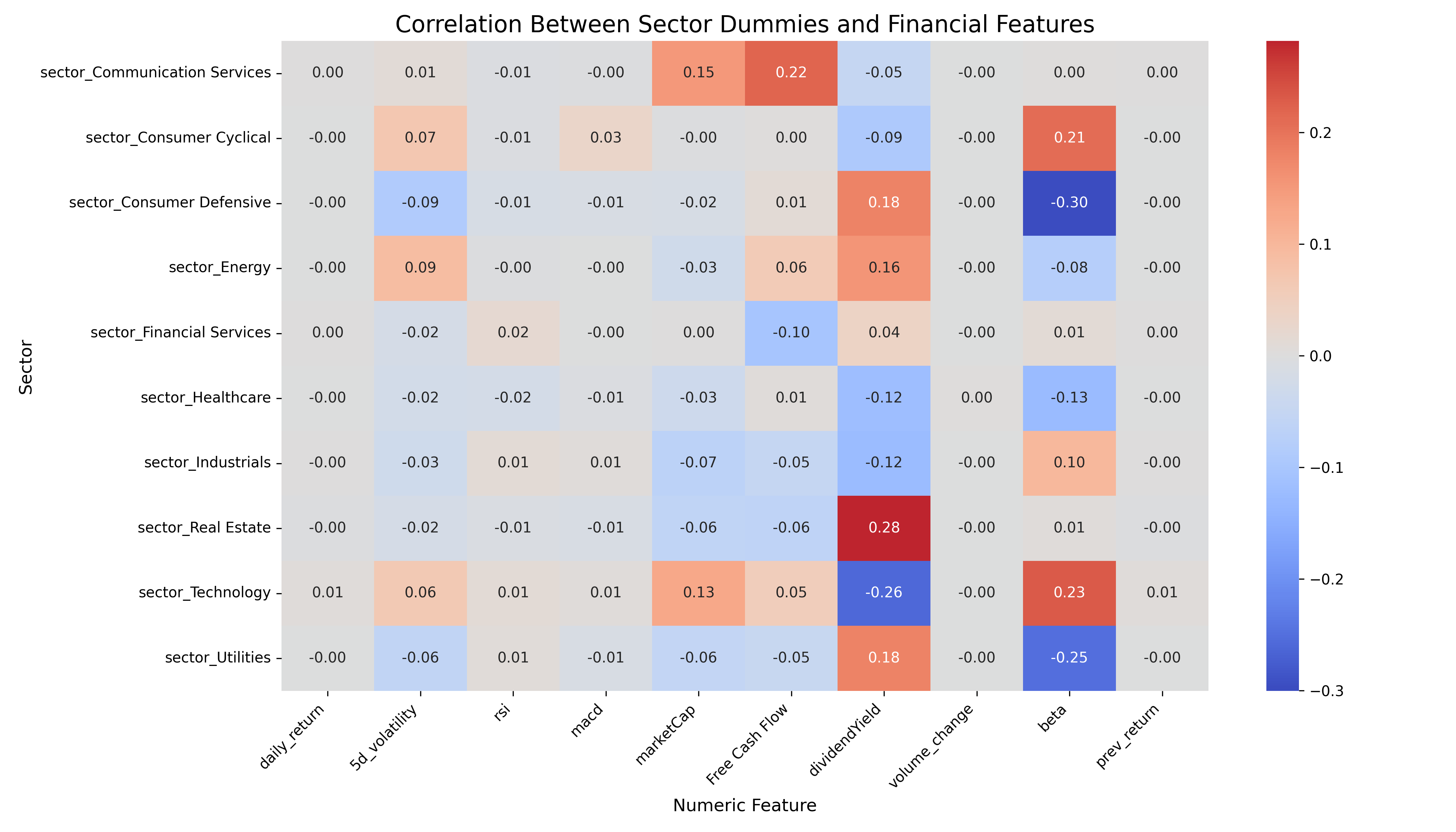
Fig. 3: Feature-to-Sector Correlation Heatmap

Principal Component Analysis (PCA): Feature Insights¶

To better understand the underlying structure of our feature space and reduce redundancy, we conducted a Principal Component Analysis (PCA). The plot below shows the top features contributing to the first principal component (PC1) — the axis that explains the greatest variance in the data.

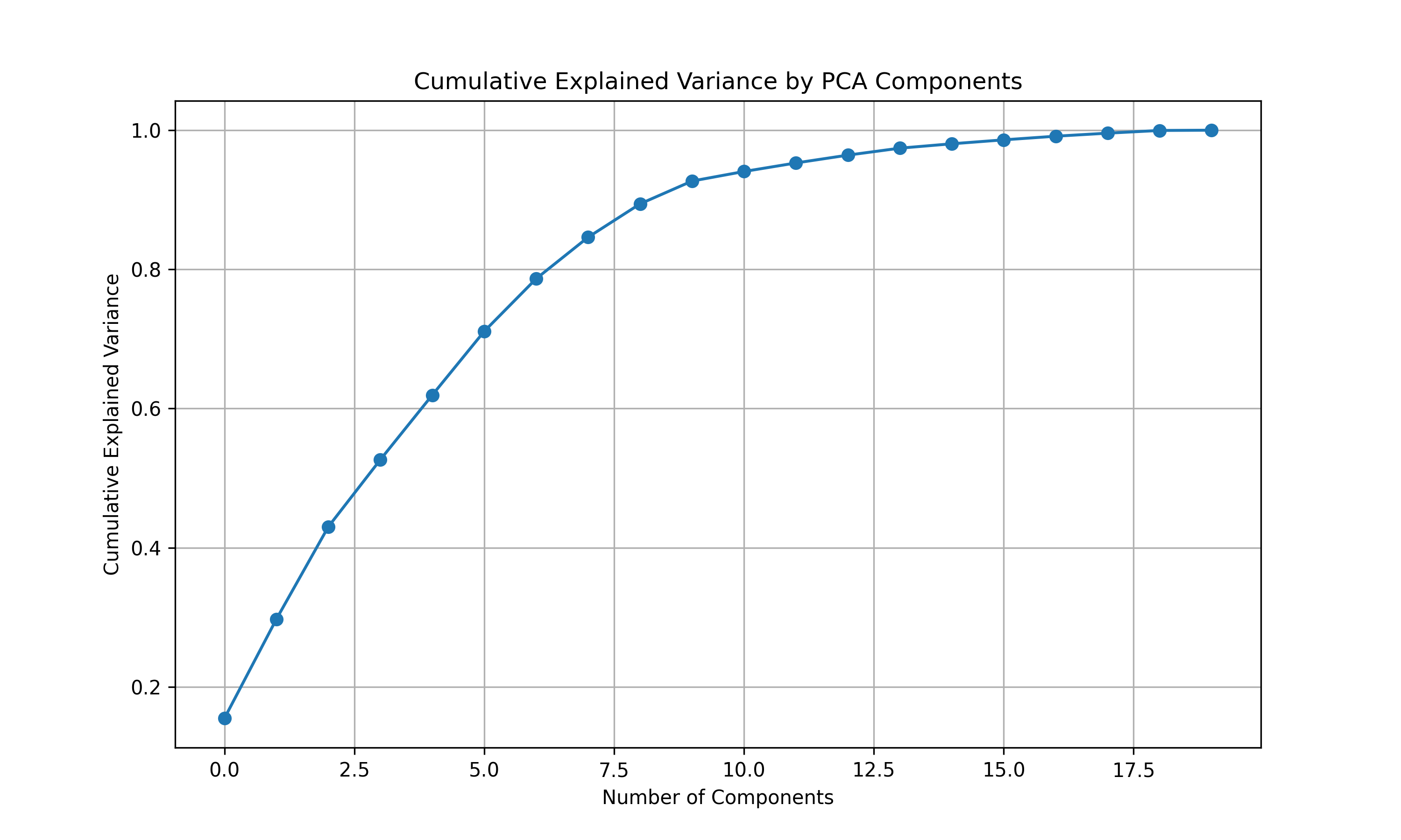
Fig. 4: Cumulative Explained Variance by PCA Components

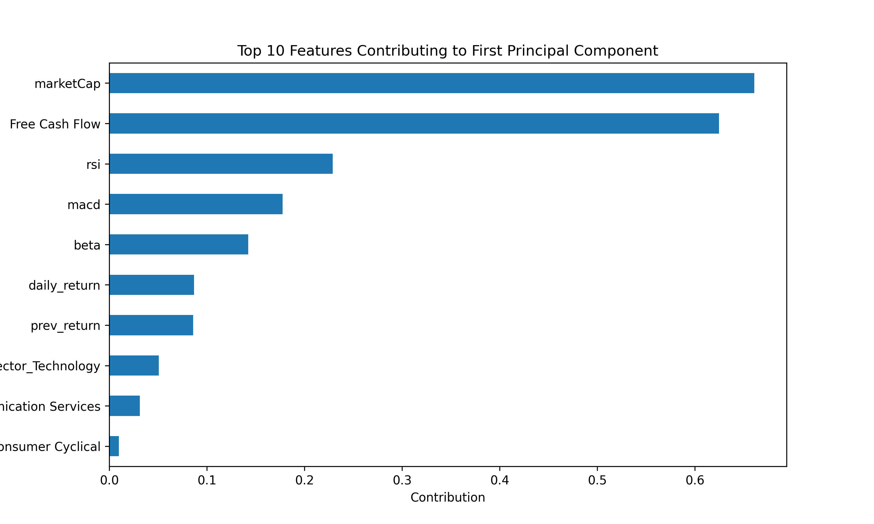
Fig. 5: Top Features Contributing to First Principal Component

The cumulative explained variance plot shows that:

The first 5 principal components capture approximately 80% of the total variance in the dataset.
Around 10 components are needed to explain 95% of the variance.
This indicates a substantial level of redundancy among the original features, making PCA a useful dimensionality reduction tool for exploratory analysis and potential model simplification.

Final Feature Selection¶

To balance predictive power, interpretability, and dimensional efficiency, our final model utilizes 20 carefully selected features, capturing a combination of technical indicators, firm-level fundamentals, and sector classification.

This selection was guided by:

PCA results, which highlighted marketCap, Free Cash Flow, RSI, and MACD as dominant contributors to the first principal component.
Correlation matrices, which revealed multicollinearity risks (e.g., between marketCap and Free Cash Flow) and clarified sector-finance relationships (e.g., Technology with high beta and low dividend yield).

Technical and Market Features:

daily_return: Recent price movement; helps capture short-term momentum.
5d_volatility: Measures short-term risk and return variability.
rsi: Momentum indicator highlighting overbought/oversold signals.
macd: Trend-following metric detecting shifts in price direction.
volume_change: Detects abnormal trading activity and liquidity signals.
beta: Captures systematic risk and sensitivity to market movements.
prev_return: Includes recent return memory while avoiding label leakage.

Fundamental Company Metrics

marketCap: Represents firm size, the strongest PCA component contributor.
Free Cash Flow: Strongly correlated with marketCap, reflects internal financial strength.
dividendYield: Indicates maturity, investor income potential, and sector defensiveness.
Sector Encoding: Sector dummy variables provide macroeconomic context, enabling the model to account for structural performance differences across industries. For example, Technology stocks typically exhibit higher beta and lower dividendYield, while Utilities are more stable and income-oriented.

This feature set reflects a well-balanced architecture, combining diverse economic signals while mitigating redundancy and overfitting risk. It is well-positioned to support accurate, generalizable classification of stock-day labels into Buy, Hold, or Sell.

Modeling Approach¶

In this section we show the calibration of four machine learning models:

Linear model: logistic regression
Non-linear models:
a. K- Nearest neighbors
b. Tree Classifier
c. Random Forest Classifier

Logistic Regression¶

In the first ML model we use a Logistic regression model to classify the stocks into either buy, hold or sell. The model learns a weight matrix $W \in \mathbb{R}^{K \times d}$, where $K = 3$ is the number of classes and $d$ is the number of features (including a bias term). The loss function we minimize combines the negative log-likelihood (cross-entropy loss) with an L2 regularization term to prevent overfitting:

$$ \mathcal{L}(W) = -\sum_{i=1}^{n} \log \left( \frac{e^{W_{y_i} \cdot \mathbf{x}_i}}{\sum_{k=1}^{K} e^{W_k \cdot \mathbf{x}_i}} \right) + \lambda \|W_{\text{no-bias}}\|_2^2 $$

To handle cross-validation and shuffuling we defined a class:DatasetManager. This class handles the preprocessing and data splitting necessary for training and testing. It takes raw features and labels, balances the dataset across classes using stratified downsampling, and then performs a train-test split to separate data for training and generalization evaluation. In our implementation we used 80% trainning and 20% test split. Additionally, we use the shuffle method to randomly permutes the training data at the beginning of each epoch, ensuring that stochastic gradient descent does not learn from data in a fixed order and thus helps improve model generalization.

To determine the best hyperparameters for our logistic regression model, we evaluated performance using both accuracy metrics and visualizations of training and test accuracy over the epochs. Accuracy on the test set allows us to assess whether the model is underfitting, overfitting, or converging as expected. Based on this evaluation, we focused on calibrating the L2 regularization strength (lambda), which penalizes large weight values to help prevent overfitting and improve generalization.

The model proved to have greater accuracy in the test set for a low lambda = 0.0001.

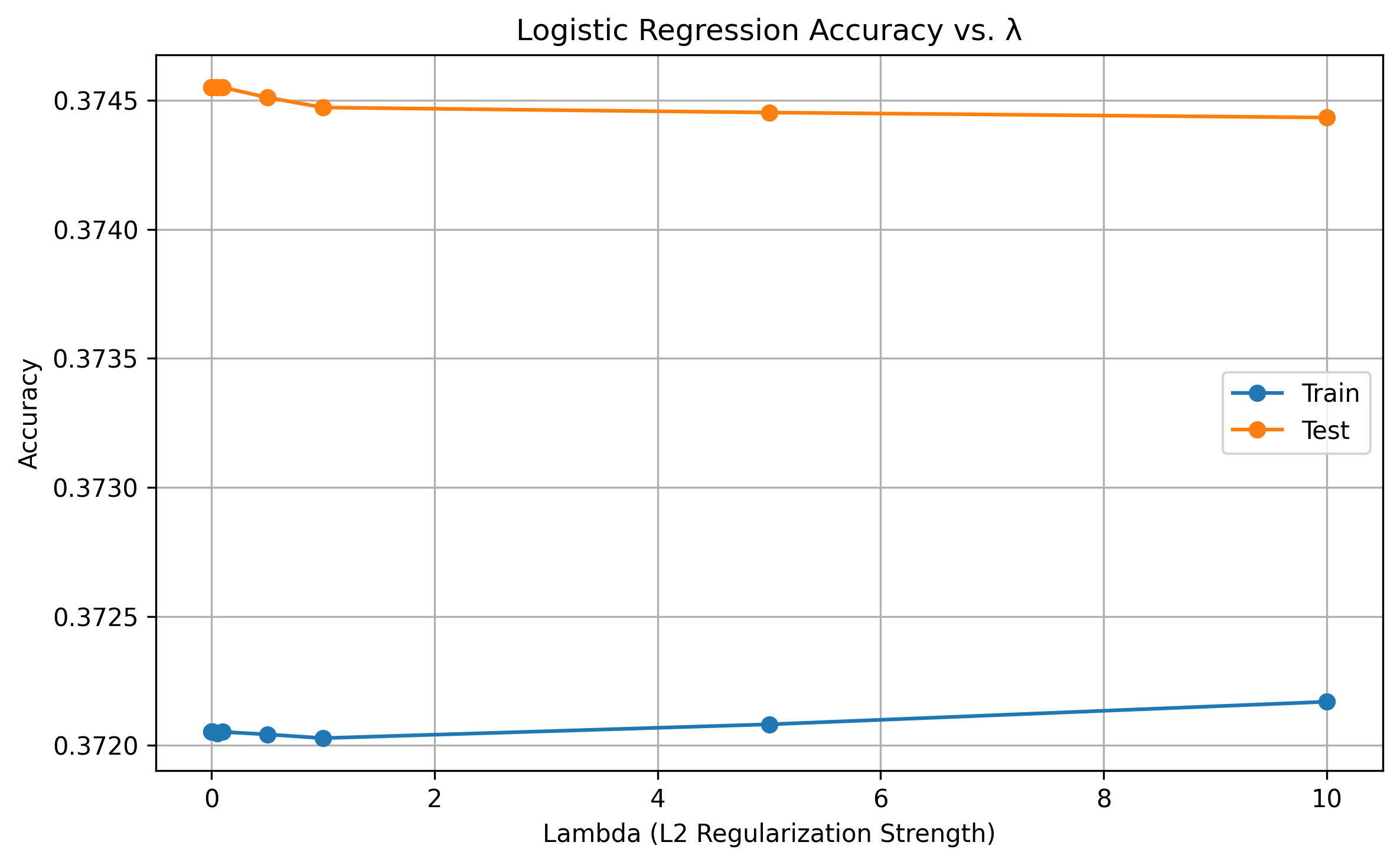
Fig. 6: Lambda Calibration

With this model we have the next confusion matrix, which predicts mostly hold and sell labels, underscoring the stocks that should be labeled as buys. This is also reflected in a low recall value for buy stocks (20.3%).

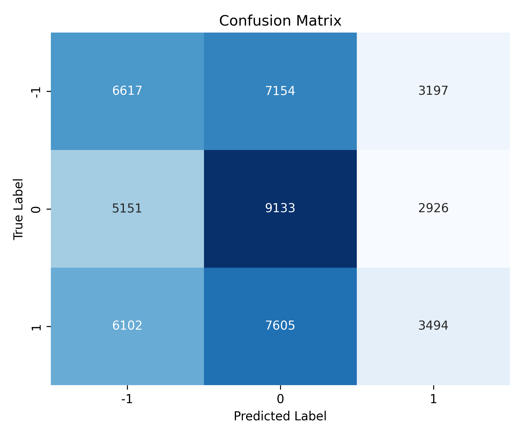
Fig. 6: Log regression confusion matrix

K-Nearest Neighbors¶

Next we experimented with K-Nearest Neighbors (KNN) initially appeared promising due to its non-parametric design, which avoids rigid assumptions about data distributions—a potential advantage in volatile markets where trends shift unpredictably. Its intuitive logic, classifying outcomes based on proximity to historical data, conceptually aligns with mean-reversion strategies, and its adaptability to both classification (e.g., buy/sell signals) and regression (e.g., price forecasting) added flexibility.

After running

!python3 ../predictions/knn_model.py

We get the results:

KNN (k=3) → Train: 0.7558, Test: 0.4195
KNN (k=5) → Train: 0.6930, Test: 0.4061
KNN (k=7) → Train: 0.6416, Test: 0.4328
KNN (k=11) → Train: 0.6136, Test: 0.4499

However, after rigorous testing, we concluded KNN was ill-suited for stock data.

Why:

The model’s high sensitivity to noise proved problematic, as single outliers skewed predictions in inherently volatile markets, while the curse of dimensionality diluted distance metrics’ relevance across our 30 financial features (price, volume, indicators).
Computational inefficiency also became a bottleneck: with 673,000+ training points, real-time predictions were impractical as KNN is a lazy learner.
Crucially, KNN’s lack of temporal awareness ignored sequential dependencies in time-series data, a fatal flaw for capturing trends or momentum.
Finally, despite meticulous feature scaling to normalize price and volume ranges, the model struggled to generalize.

While KNN’s simplicity and assumption-free structure offered theoretical appeal, its limitations in handling noise, scale, time sensitivity, and high-dimensional financial data ultimately led us to prioritize alternative models.

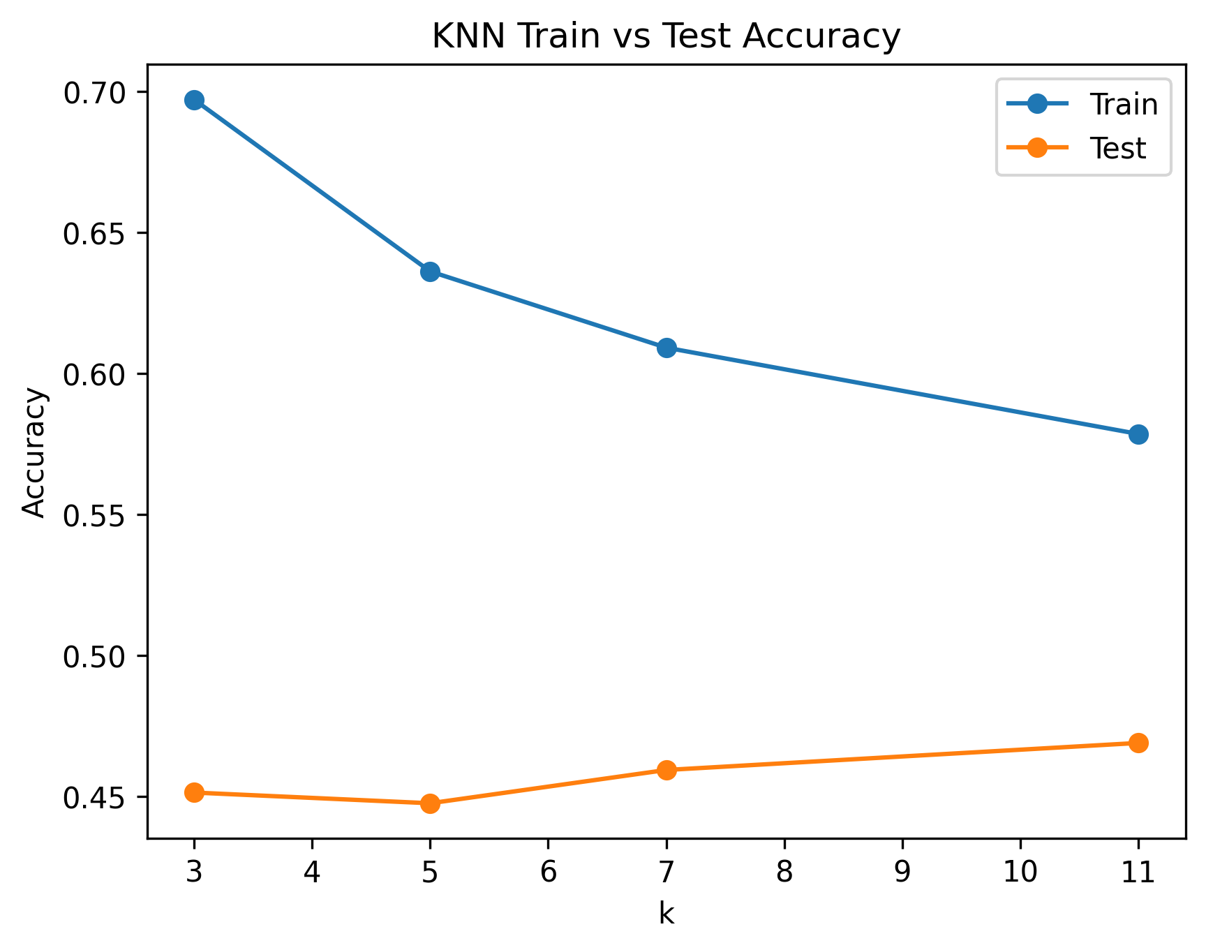
Fig. 7: KNN Train vs Test Accuracy as a function of k

Tree Classifier¶

Third, we implemented a decision tree classifier, a supervised non-linear model, to predict stock labels as buy, hold, or sell based on the same financial and sector-related features. The model is trained using a recursive, top-down approach that splits the data at each node based on the feature and threshold that maximizes information gain. As impurity measure we used entropy, which is the measure to classify the proportion of each category and the log function as follows:

$$ H = -\sum_{i=1}^C p_i \log_2(p_i) $$

where C are the categories and $p_i$ the proportions of each category.

Information gain uses the impurity difference from the parent node and the children nodes as follows: $$ Information\;gain = H(parent) - [\sum_{i=1}^n p_i H(child_i)] \\\ H(D) - [p_1 * H(D1) + p_2 * H(D2)] $$

where n is the number of child nodes.

The primary hyperparameter tuned in the decision tree was its depth, trying depths of [3, 6, 9, 12, 15, 21]. The highest accuracy of the tree with the 21 variables is reached for a depth of 12 nodes, with an accuracy of 0.3755.

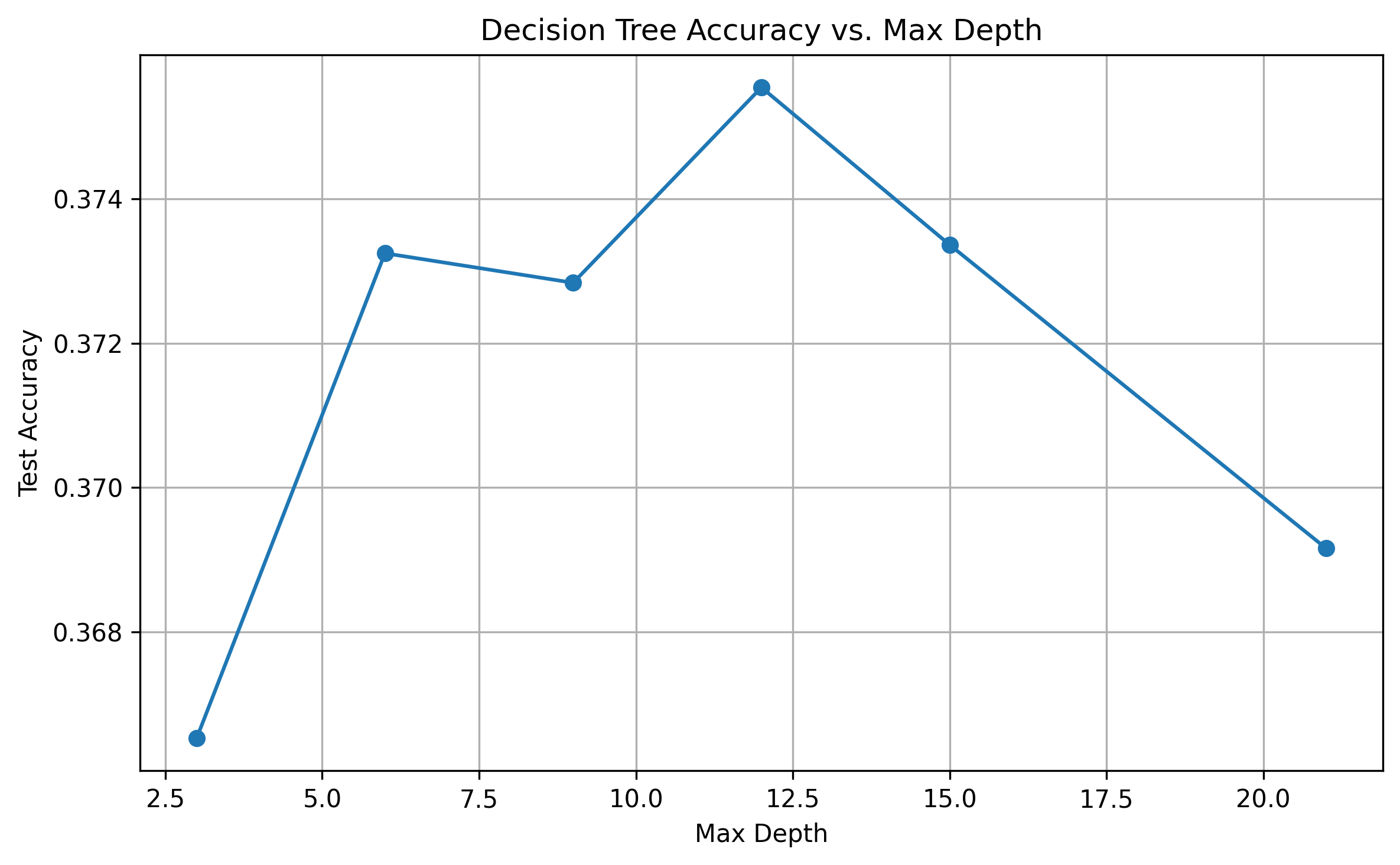
Fig. 8: Decision Tree Accuracy vs. Max Depth

The main contributors to the tree explainability are MACD, RSI and Beta, while the sector of the companies have the lower predictive power.

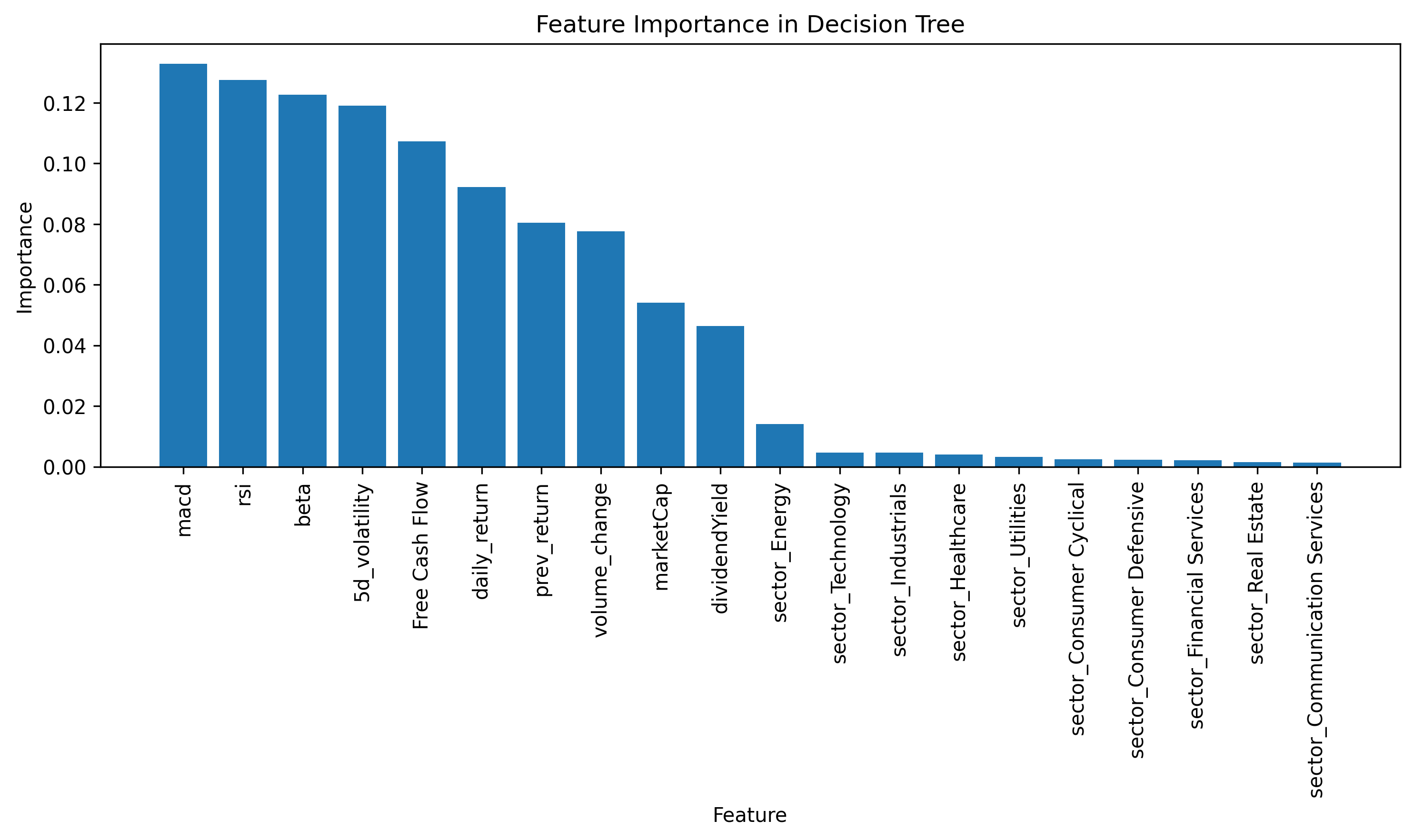
Fig. 9: Decision Tree contributors

In this context the confusion matrix shows that the model correctly predicts most holdlabeled stocks, but still has a low recall for buystocks (23%).

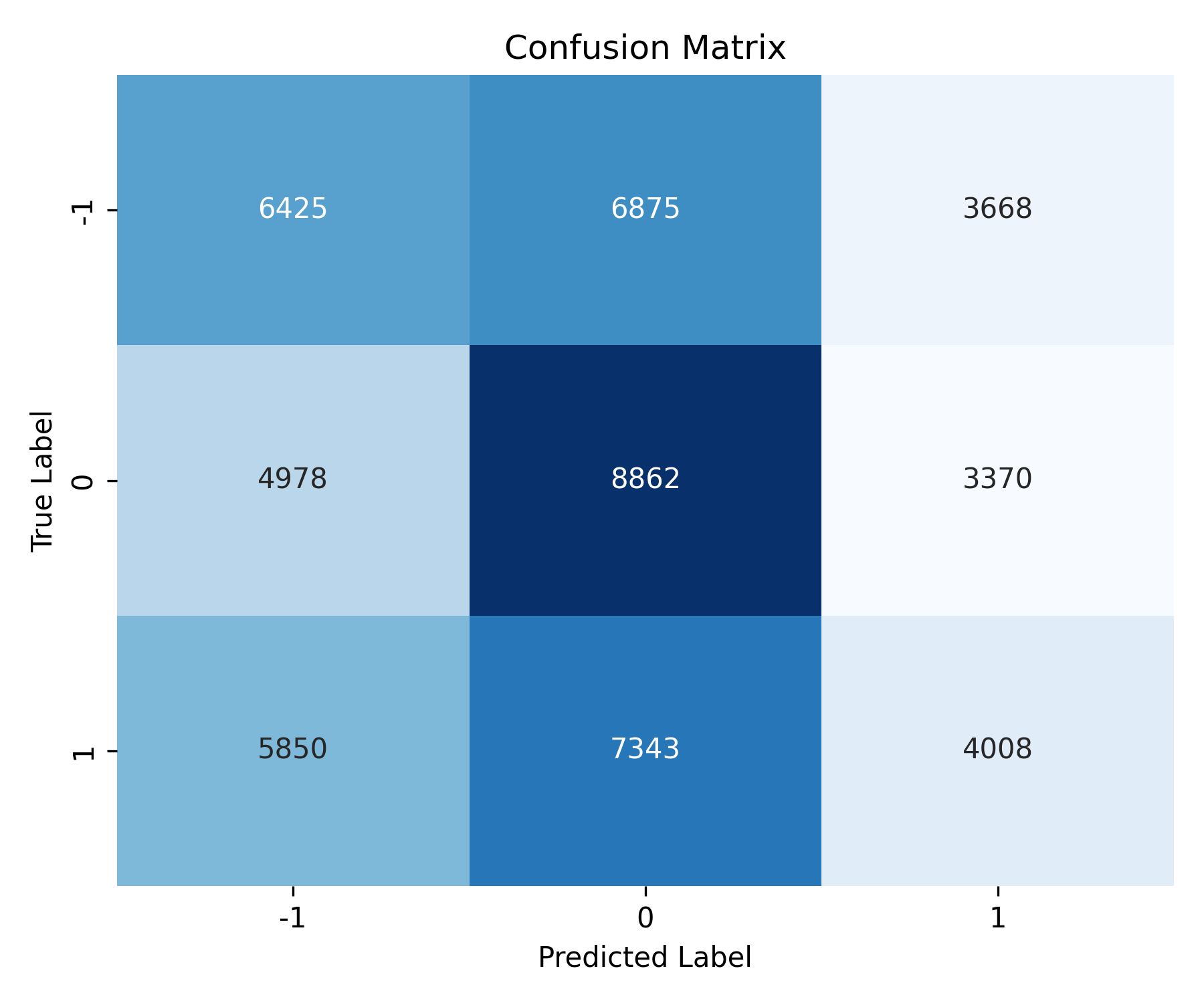
Fig. 10: Decision Tree Confusion Matrix

Random Forest Classifier¶

To evaluate classification performance in a high-dimensional, mixed-type feature space, we employed a Random Forest Classifier—a robust, non-parametric ensemble learning method.

Random Forest is particularly well-suited for this task because:

It handles heterogeneous features seamlessly (technical indicators, fundamentals, and categorical dummies).
It mitigates overfitting through bagging and feature randomness.
It captures non-linear interactions and higher-order feature relationships that linear models may miss.
It provides feature importance scores, allowing interpretation and variable selection.

These properties make Random Forest an excellent benchmark model for evaluating the predictive structure in our dataset.

In our pipeline, Random Forest is not only used for classification, but also as a diagnostic tool to:

Quantify feature relevance using Gini-based variable importance.
Benchmark accuracy, precision, recall, and F1-score against simpler models (e.g., logistic regression).
Assess stability under variations in random seed, train/test splits, and class balancing.

We systematically tuned five key hyperparameters using manual grid search and performance visualization:

n_estimators: Number of trees in the ensemble.
max_depth: Maximum depth of each tree (controls complexity).
min_samples_split: Minimum samples required to split a node.
min_samples_leaf: Minimum samples required at each leaf (final prediction).
max_features: Fraction of features considered at each split.

We fixed class_weight='balanced' to address the natural class imbalance in our Buy/Hold/Sell targets and ran all models with random_state=30254 and n_jobs=-1 for reproducibility and efficiency.

Tuning was carried out using training/validation folds and test set holdout evaluation.

The Random Forest classifier aggregates predictions from ( T ) decision trees:

$$ \hat{y} = \frac{1}{T} \sum_{t=1}^{T} h_t(x) $$

Where:

$h_t(x)$: prediction of the ( t )-th tree
$T$: total number of trees
$\hat{y}$: final prediction (majority vote for classification)

This ensemble approach increases robustness and reduces overfitting by averaging across uncorrelated trees.

In summary, Random Forest provided a powerful and interpretable model for our financial classification task, combining strong performance with valuable diagnostics for feature selection and model robustness.

Hyperparameter Tuning

All tuning results are visualized below:

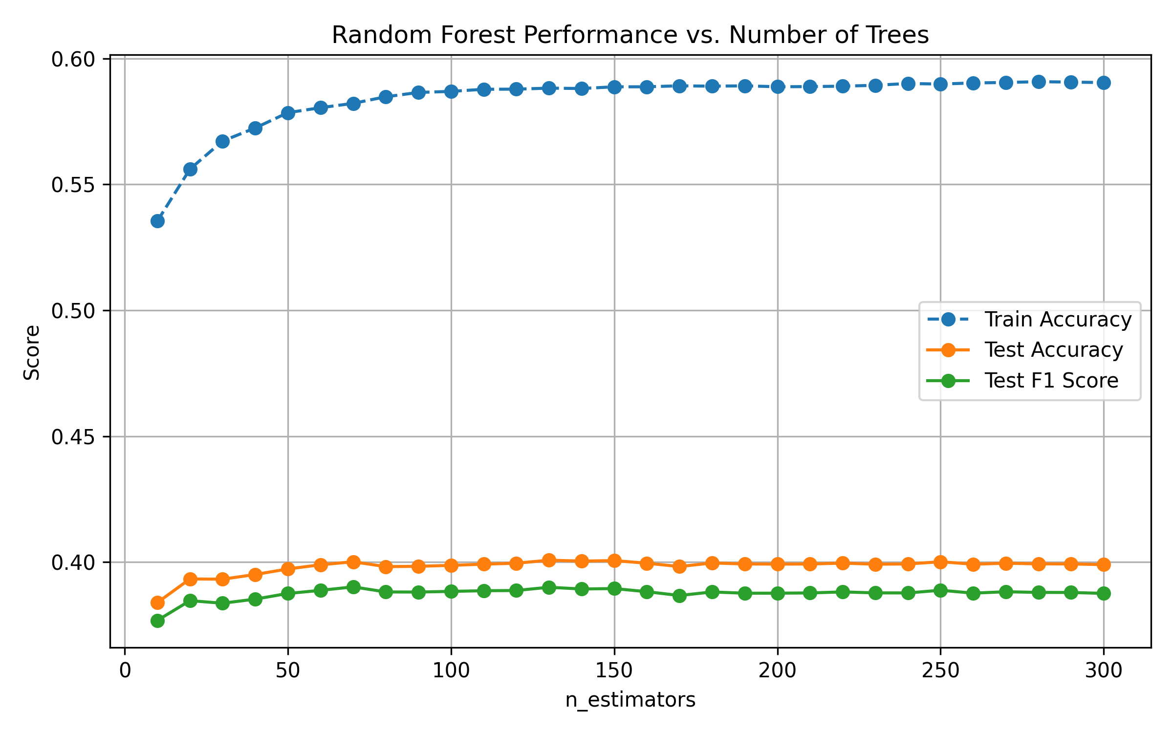
No description has been provided for this image

Fig. 11: Test Accuracy and F1 vs. Number of Trees

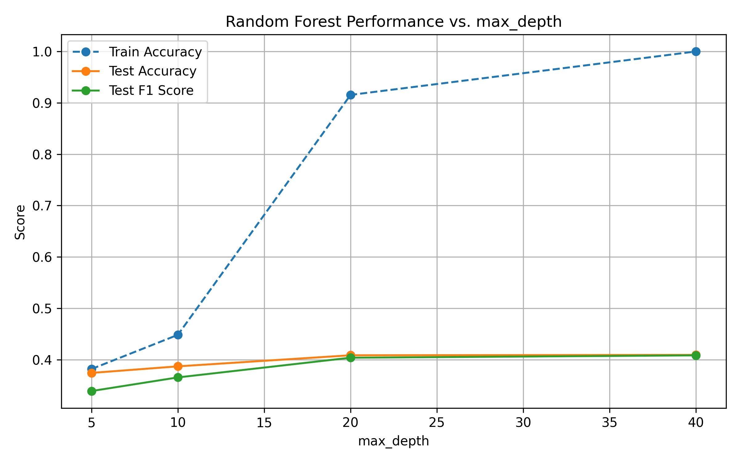
Fig. 12: Performance vs. Tree Depth

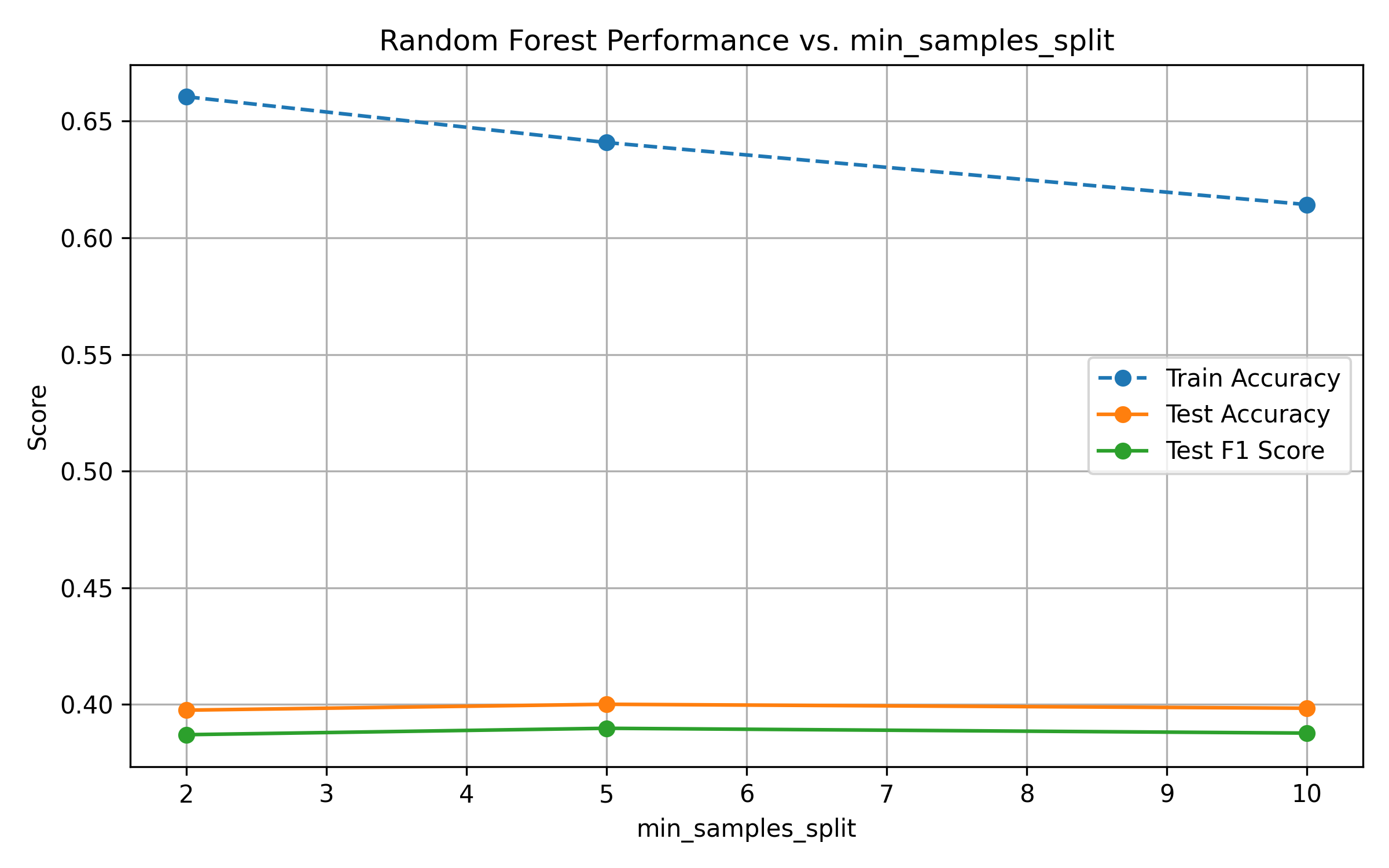
Fig. 13: Performance vs. Minimum Samples per Split

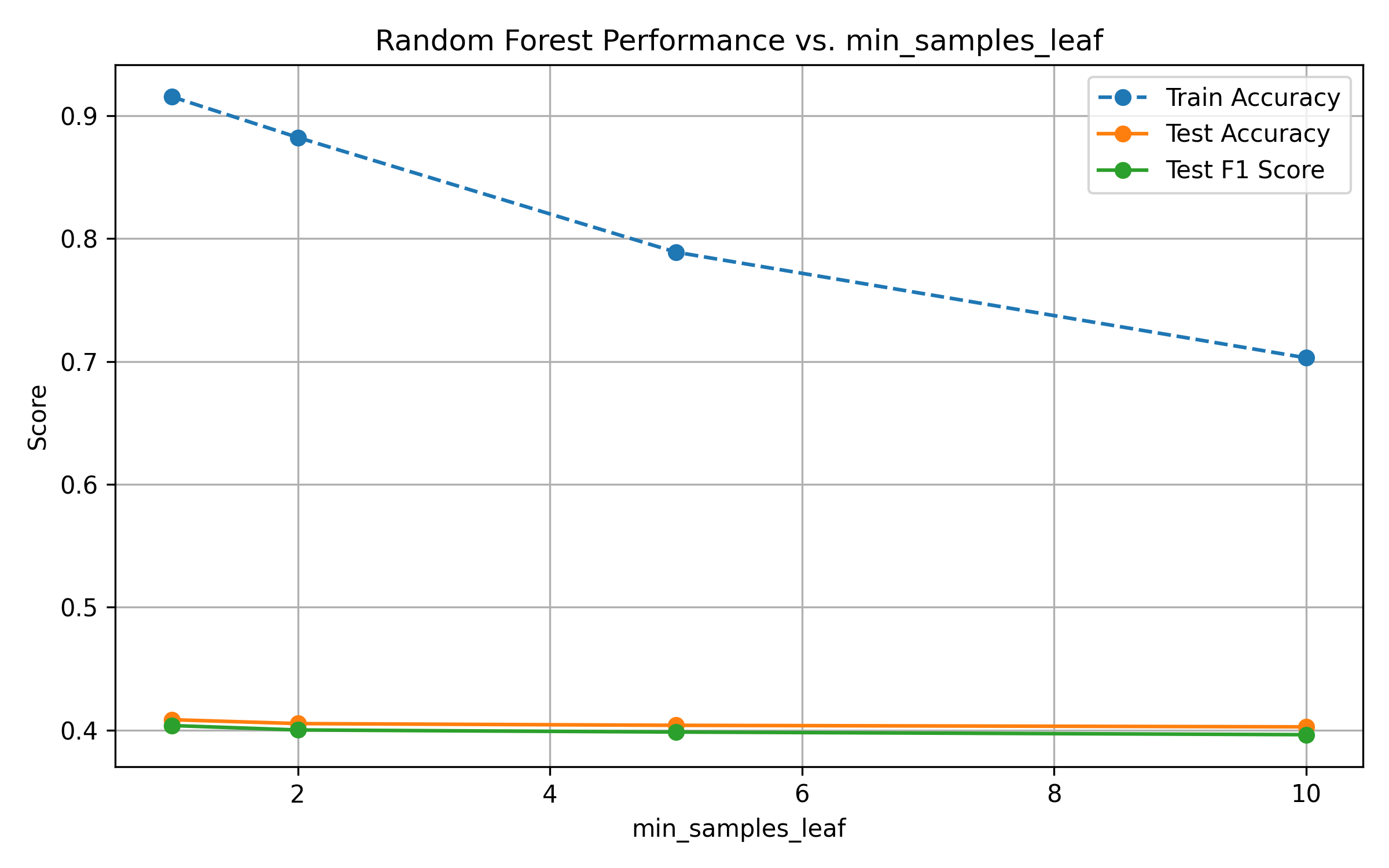
Fig. 14: Performance vs. Minimum Samples per Leaf

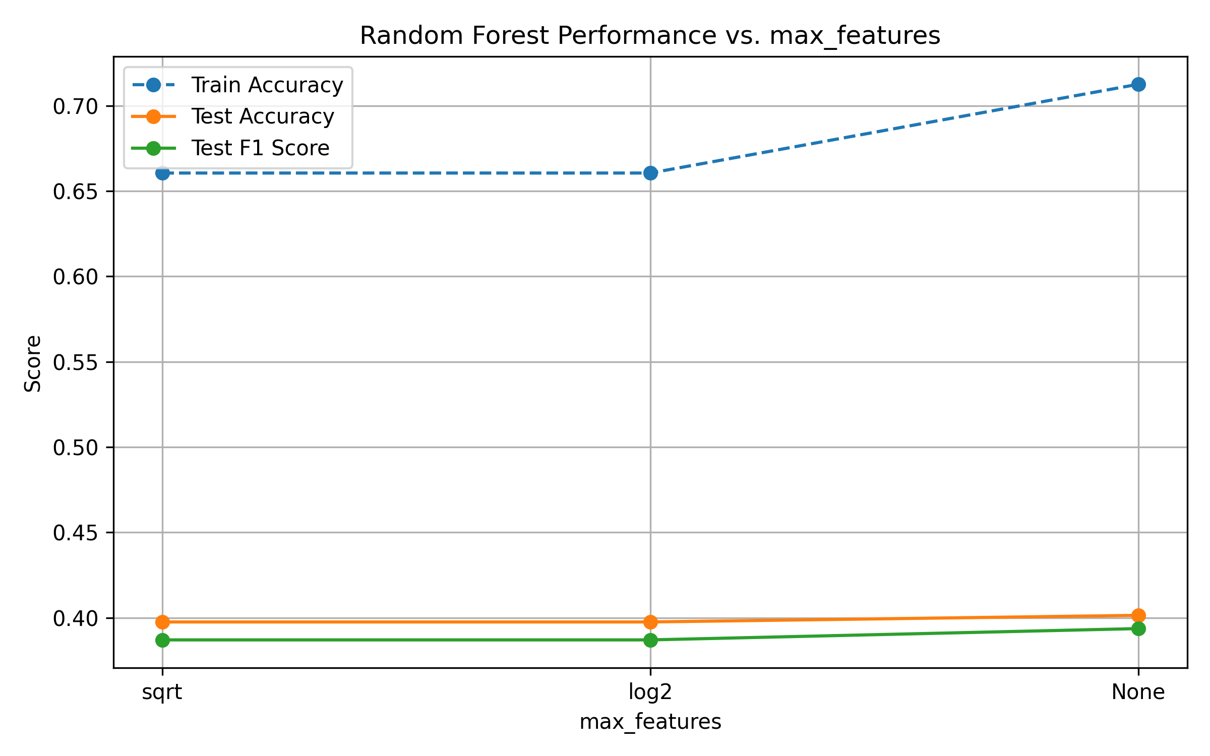
Fig. 15: Performance vs. max_features

Increasing n_estimators improves test performance, but returns diminish after 200–300 trees.
Increasing max_depth leads to overfitting: train accuracy reaches 1.0, while test metrics plateau.
Higher values of min_samples_split and min_samples_leaf reduce model complexity. While this constrains overfitting, gains in generalization are marginal—performance remains stable.
Across all parameters, test F1-score provides a more balanced view of performance than accuracy, reflecting the effects of class imbalance.
Train accuracy reaches 100% early, highlighting the model's capacity.
Test metrics plateau across all hyperparameters, suggesting the presence of data noise or irreducible error.
F1-score gives a more nuanced picture than accuracy due to class imbalance.

After hyperparameter tuning and evaluation on the holdout test set, the final Random Forest model achieved a macro-averaged F1-score of 0.408 and overall accuracy of 41.3%. The confusion matrix and classification report provide deeper insights into class-level performance.

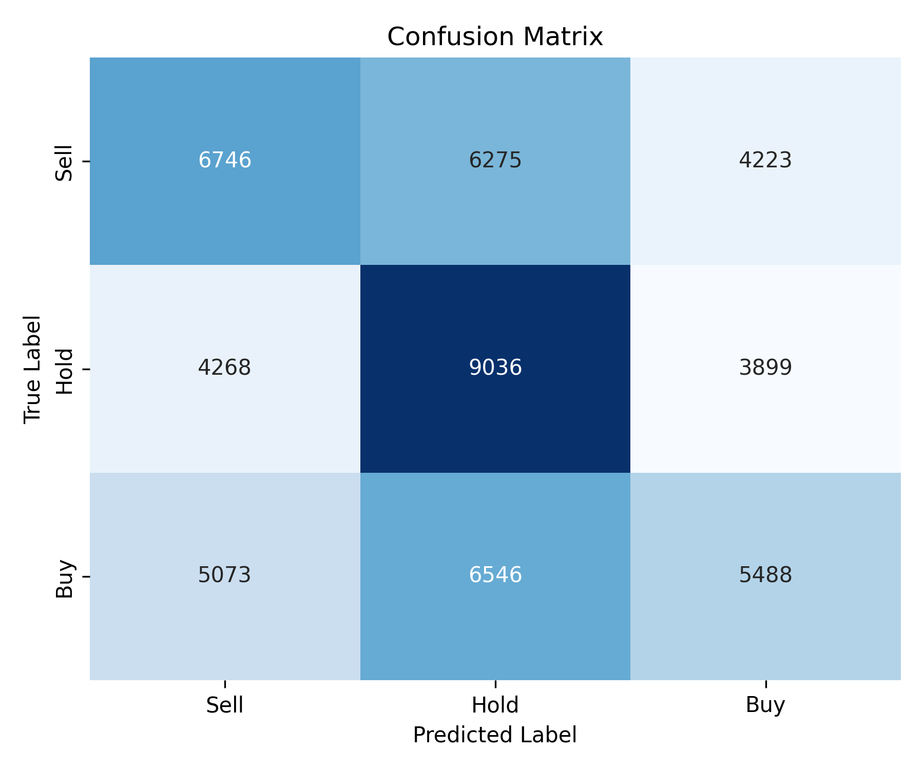
Fig. 16: Test Accuracy and F1 vs. Number of Trees

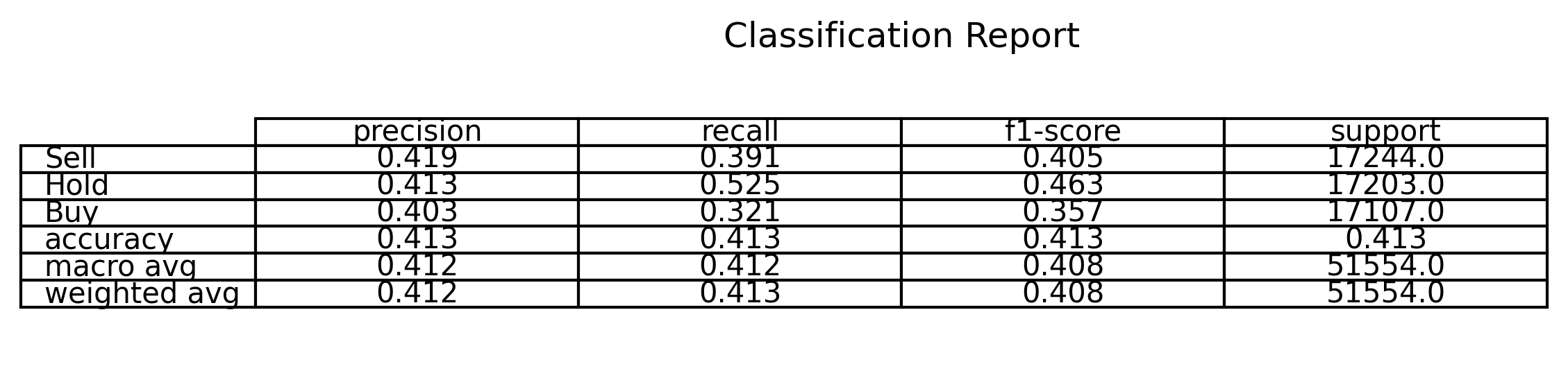
Fig. 17: Performance vs. Tree Depth

The "Hold" class was predicted with the highest recall (52.5%), indicating the model's relative strength in capturing moderate return conditions. In contrast, the "Buy" and "Sell" classes showed lower recall and F1-scores, reflecting the challenge of separating outperforming and underperforming stock-days based on financial indicators alone. The confusion matrix revealed that:

Misclassifications between Buy and Hold are frequent, suggesting overlapping features or market ambiguity.
The model tends to slightly overpredict Hold, which is common in imbalanced or uncertain financial classification tasks.

Random Forest served as a strong baseline for performance and feature interpretability. Its resistance to overfitting, ease of training, and diagnostic clarity make it a valuable component of our modeling toolkit—especially in the early and exploratory phases of financial prediction.

Key benefits included:

Robustness to mixed datatypes and noise
Integrated feature importance measures
Scalability across parallel CPU environments

Challenges and Limitations¶

A key methodological challenge in this project was the implementation of custom machine learning algorithms from first principles. While instructive, developing our own logistic regression, k-nearest neighbors, and decision tree classifiers proved computationally intensive and less efficient than established libraries such as scikit-learn. The absence of built-in optimization and validation routines required significant manual calibration and increased the risk of implementation errors, particularly for non-parametric models like KNN and decision trees.

Beyond computational constraints, our results underscore fundamental limitations in applying standard classification models to financial market data. Stock returns are characterized by high volatility, non-stationarity, and autocorrelation—features that violate the independence assumptions of many supervised learning algorithms. Moreover, the decision boundary between “Buy,” “Hold,” and “Sell” is rarely linearly separable. These characteristics contribute to the difficulty our models faced in generalizing beyond the training set, particularly in capturing rare but economically meaningful signals such as buying opportunities.

These challenges highlight the importance of model selection and data structure in financial prediction tasks. In future work, integrating time-aware architectures and broader information sets may be necessary to overcome these structural constraints.

Conclusions and future work¶

This work implemented and calibrated four machine learning classification models—logistic regression (custom and scikit-learn), decision trees, and k-nearest neighbors—to classify daily stock-level observations into investment signals: Buy, Hold, or Sell. While model performance varied modestly across specifications and tuning parameters, a consistent pattern emerged: recall, particularly for the “Buy” categories, remained low across all models. This suggests that even well-calibrated classification algorithms struggle to consistently identify profitable trading signals in high-frequency, firm-level stock data.

These findings are consistent with the broader empirical literature that highlights the difficulty of outperforming the market using past returns and financial indicators alone. Stock price movements are known to exhibit significant noise, nonlinearity, and autocorrelation—characteristics that are not easily captured by standard machine learning classifiers assuming i.i.d. observations. Consequently, while accuracy metrics may suggest moderate in-sample fit, the models' out-of-sample predictive power for economically relevant signals is limited.

Future work should explore models explicitly designed to capture temporal dependence and nonlinear structure in time series data, such as recurrent neural networks (e.g., LSTMs) or sequence-to-sequence transformers. Additionally, incorporating richer information sets—such as macroeconomic indicators or news sentiment to improve the signal-to-noise ratio and yield more actionable investment strategies.